11.7.1 Norway

Introduction

The following report describes the workflow for calculation of indicator 11.7.1 within the framework of the GEOSTAT 3 project, work package 2, by Statistics Norway.

We have calculated indicators based on the following data and concepts:

A national proxy indicator on the population’s access to recreational (green) areas
Test-calculation of the population’s access to green and open spaces based on the Urban Atlas data

a. Following methodology similar to Dijstra and Poelman, and

b. By proportion of population within 200 metres around such areas

3. Test-calculation of the populations access to open spaces based on GHSL BUILT-UP

a. In combination with GHSL population

b. In combination with national grid population

c. In combination with address point population

Data status

Population data from the National Registry[1] geocoded to address point location: The National Registry, under the responsibility of the Norwegian Tax Administration, can be geo-enabled by use of geocoded authoritative address and/or building data from the NMCA (Kartverket). Statistics Norway has a “statistical copy” of the National Registry, updated on a daily basis, hence geocoded population can be obtained for any point of time. Data for the year 2016 has been used.
Geographic delimitation of urban areas (localities – urban settlements) following national methodology, produced by Statistics Norway: Data on localities is national authoritative data available under open data licenses. Data for the year 2017 has been used.
Urban and High-density cluster grid from Eurostat based on the GEOSTAT 2011 population grid: Data for the year 2011 has been used.
GHSL – Global human settlement layer 2015: Data on built-up and population based on satellite imagery and other sources.
Roads and paths from national roads database as well as detailed municipal maps, made available through the national geospatial infrastructure (Geonorge https://www.geonorge.no/en/about/what-is-geonorge/).
Copernicus Urban Atlas land use/ land cover classification (2012) exists for 6 of the larger city areas in Norway. In this test, we have made statistics for the 4 high density clusters in Norway.

Processes

We have tried out different methodologies in addition to the national proxy indicator. This is to highlight differences and similarities between data sources. Can more simplified approaches suffice? On a national level or on regional level?

In the testing for Norway of indicator 11.2.1 we saw that population figures for urban clusters were quite similar to the nationally delimitated urban settlements (=> 5 000 residents), but on more detailed level differences are bigger.

a) Geocoding population data

The “statistical copy” of the national population register at Statistics Norway includes references to address, dwelling ID and Real property ID at unit record level (e.g. at the level of each individual unit). Data is collected by the Tax administration and transferred on a daily basis to Statistics Norway. Hence, geo-enabling population to address location is quite straightforward and can be deployed for any point in time using the authoritative address register from the NMCA. A copy of the address register is kept in Statistics Norway and the location of each address is stored as attribute information in the statistical databases (Oracle technology). Extracts are made regularly for unit record data with building location and address location. Address location with aggregated population by age and sex is served as a geometry table and feature class for use in desktop GIS software.

Some 99.8 percent of the population can be directly geocoded to the level of address location. For different reasons the remaining 0.2 percent cannot. The remaining 0.2 percent represents individuals without a permanent place of residence (homeless people, prisoners and elderly people in special care centres etc.) and cannot be more accurate geo-located than to the municipality in which they were registered. In order to obtain a full geocoded record, different location objects are used. Metadata at the level of each individual record describes the matching type and quality according to a fixed coding system. See table below. Codes A and B give exact address coordinate, while C gives neighbouring address. When conducting the calculations, only population assigned to address location is regarded.

Table 1: Metadata describing geocoding quality at unit record level

Quality Code	Number of people geocoded	%
A1 – Address 21 pos	5 272 662	99,6
A2 – Address 17 pos	382	0,0
A3 – Address 13 pos	1 133	0,0
B1 – Address (old) 21 pos	8 082	0,2
B2 – Address (old) 17 pos	23	0,0
B3 – Address (old) 13 pos	7	0,0
C1 – Address ± 1	163	0,0
C2 – Address ± 2	63	0,0
C3 – Address ± 3	18	0,0
C4 – Address ± 4	6	0,0
C5 – Address ± 5	17	0,0
C6 – Address ± 6	9	0,0
No geocoding	13 054	0,2
Total population	5 295 619	100

b) Delimitation of urban agglomerations:

In principle, this step has already been completed prior to the indicator analysis. Two different concepts/data sources have been tested:

Classification of urban areas based on national data (Norwegian “urban settlements”).
Classification of urban areas on European data on high-density and urban clusters (using data from Eurostat based on the grid cluster method).

Statistics Norway has recurrently delineated the geographical extent of urban areas (“urban settlements” or “localities”) as part of the production of official urban statistics since the 1960 census. Digital boundaries are produced annually since 2000. A locality consists of a group of buildings normally not more than 50 metres apart and must fulfil a minimum criterion of having at least 200 inhabitants. Thus, localities include the largest cities as well as small settlements with 200 inhabitants as the lower threshold. The delimitation is conducted as an automated workflow involving high quality authoritative geospatial data from the NSDI in combination with point-based population data geocoded to the level of address location. The result is a national polygon dataset representing the urban extent of each locality (some 1 000 in Norway). Data is available under open data license agreements https://kartkatalog.geonorge.no/metadata/statistisk-sentralbyra/tettsteder-2017/9b4fdbcb-d682-4cea-8e10-e152bbeb481e ).

To enable comparison between national and European data, a cut-off has been applied to the national data, taking into account only those urban clusters in national data having 5 000 inhabitants or more.

Converting Urban clusters and high-density clusters

The clusters are 1 km grids with contiguous (8 neighbours), grids with at least 300 inhabitants in each grid cell, at least 5 000 in all to qualify for urban cluster. High density grids are similarly identified by at least 1 500 inhabitants in each grid cell and a minimum of 50 000 in the cluster as a whole (4 neighbours connectivity). For this indicator 2011 data was used.

The clusters can be downloaded from Eurostat: http://ec.europa.eu/eurostat/web/gisco/geodata/reference-data/population-distribution-demography/clusters.

Pre-processing included extracting data for Norway, projecting to UTM 33 ETRS89 and converting to vector format.

Identifying open space based on GHSL in combination with urban clusters

The Global Human Settlement (GHS) framework produces global spatial information about the human presence on the planet over time. This in the form of built up maps, population density maps and settlement maps. This information is generated with evidence-based analytics and knowledge using new spatial data mining technologies. The framework uses heterogeneous data including global archives of fine-scale satellite imagery, census data, and volunteered geographic information. The data is processed fully automatically and generates analytics and knowledge reporting objectively and systematically about the presence of population and built-up infrastructures.

The general methodology behind GHSL data introduces concepts of GHS BUILT-UP, GHS POP, and the GHS Settlement Model. The main datasets are offered for download as open and free data.

The data consists of multitemporal products that offers an insight into the human presence in the past: 1975, 1990, 2000, and 2014. See http://ghsl.jrc.ec.europa.eu/index.php.

In the testing we have used the GHS BUILT-UP which has information layers on built-up presence as derived from Landsat image collections (GLS1975, GLS1990, GLS2000, and ad-hoc Landsat 8 collection 2013/2014). A quality grid for the built-up (GHSL BUILT-UP QUALITY) has also been studied, as well as the population grids (GHSL-POP).

Although GHSL built-up exists for almost all of Norway for the different years (see appendix 1) it has some obvious weaknesses. In part agricultural areas are classified as built-up. The same is the case for some forest areas and gravel/ bare rock areas. This is noticeable in western parts of Norway as well as in parts of northern Norway. The cities of Trondheim and Tromsø are not represented with built-up in a reliable way. See appendix 1 for some figures illustrating properties of the data. Despite this, we have used the data for testing purposes. Because of the quality issues we could not have used the data for ordinary statistical production at the present time, and there exist other options for Europe (although not with such a long time series – Copernicus products).

In this approach we use Urban clusters and High-density clusters based on GEOSTAT 2011 in combination with GHSL 38 m built up. “Open areas” are defined as: Urban – (built-up + water). Population figure are calculated based on both the population from GHSL 2015 (250 m grid) and population from national grid (250 m), as well as point based address population.

Pre-processing included extracting data for Norway, projecting to UTM 33 ETRS89 and converting to vector format. ArcGIS Modelbuilder production lines where set up for this task.

Compiling land use/ land cover dataset

Statistics Norway compiles a land cover/ land use data set every year. Land use statistics is made possible through exchange of geodata via the National geospatial infrastructure (Digital Norway cooperation – coordinated by the NMCA) as well as agreements between SN and the NMCA and others regarding data quality feedback and delivery.

In order to produce cost-effective land use statistics covering all of Norway, existing cartographic databases and registers, including the classifications/nomenclature these are based on, must be used. Statistics Norway has created a hierarchical classification system, “Standard for classification of land use and land cover”, which is mainly based on existing standards and nomenclatures (www.ssb.no/en/klass/).

The method applied is based on utilising the highest quality data sources available, but where no optimal data source exists, the next best quality data sources are used. In practical terms, the method is an automatic geographic information system (GIS) that defines, classifies and assembles the data into a hierarchy.

In the statistics on land use and land resources all areas with buildings are classified as built-up. In addition, the building types within a built-up area determine the classification of that area. The built-up area can be made up of one ground property, part of a property or the area immediately surrounding the building. A property can be made up of several separate built-up areas that are classified individually.

In order to produce the data set where buildings determine the land use, a number of data sets need to be used: land resource map, properties, roads, water and coastlines, in addition to building points from the Cadastre and the building outlines. The methodology used to adapt built-up areas and calculate the utilisation rate is shown in Figure 1.

Figure 1. Land use map. Methodology sketch.

	The land resource map AR-STAT (1: 5 000 in urban-areas), in which land is divided into polygons based on land type, is used to define built-up areas. When defining built-up land, the land types “built-up” and “open firm ground” (firm ground that is not agricultural land, forest, built-up or traffic areas) are the primary land types since both can define the built-up part of a property.
	The land resource map is simplified by merging undeveloped land categories, and is assembled using a digital property map. Road areas are removed from the data source. Some properties only contain one land type and are treated as a whole property, while properties with more than one land type are broken down into parts of properties that are treated individually with regards to land use in the onward process.
	Buildings are included and the utilisation rate is calculated for each property or part of property. The utilisation rate is the base area of the buildings as a ratio of the built-up area. Where a property consists of both built-up and other land, a utilisation rate is calculated for both the built-up area and for the remainder of the property.
	Properties and parts of properties are classed as built-up if the utilisation rate is high enough. In general, the utilisation rate must be at least 4 per cent. The shaded areas are classified as built-up in this housing estate.

For further information on the methodology see https://www.ssb.no/en/natur-og-miljo/statistikker/arealstat/aar. See also https://kartkatalog.geonorge.no/metadata/statistisk-sentralbyra/arealbruk/a965a979-c12a-4b26-90a0-f09de47dbecd.

Identifying potential recreational areas (green areas)

Based on the land use/cover geodatabase and data on roads and paths which is served as part of the National geospatial infrastructure, Statistics Norway identifies potential recreational areas and the population with access to such areas, and publishes statistics every second year.

There is no nationwide mapped information on recreation area. It was therefore chosen to identify areas that may have potential as a recreational area.

The following areas are included in recreation areas (from Statistics Norway’s land use/cover map):

Forest, open solid ground, wetlands, bare rock, gravel and boulder fields, parks and sports fields cf. Statistics standard classification of areas for statistical purposes (www.ssb.no/en/klass/).

Lakes and ponds that are less than 1 acre are also included.

Sports facilities that are not normally available for public recreational activities are not included.

When areas are identified and delineated, some adjustments are made to the areas for the size to be calculated as correct as possible:

Potential recreation areas adjacent to each other, but which are separated by narrow built-up areas or areas of communications, are merged as long as they are closer than 5 meters. That is, we consider these areas as part of a larger area, even if it is intersected by other narrow land use classes. This is significant for which recreational areas that meet the size criteria.
Potential recreational areas that are less than 10 meters wide are also weeded out as this is largely land between roads or in relation to roads. Such areas have often limited value for recreation .

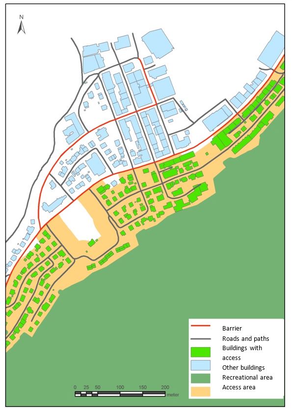
Access calculation is done by calculating the distance along the roads, footpaths and cycle paths and trails. One is considered to have access if within 200 m from recreational areas. Safe access is calculated as: If you do not have to cross a road with relatively heavy traffic or over a certain speed limit (annual average daily traffic of 3 000, speed limit 30 km./h). In addition, railroads are considered as a barrier (see figure 2). Criteria are set for children’s safe access.

Figure 2. Identification of access to recreational areas

First, paths and roads which can be traversed and crossed safely, are identified.

Then barrier roads are identified.

Calculate distance along roads and paths (200 metres for recreational areas). One is not allowed to cross barrier roads in the same plane.

Make access areas by:

1) Recreational areas get an addition of 30 metres to include people living in the immediate vicinity to these areas, and

2) Adds a standard buffer distance on each side of access roads and paths of 30 metres (the roads are in addition represented by 10 metres standard with).

Buildings and resident (address) population within access areas are identified from which statistics are made.

The land class from the land resource map AR-STAT “open solid ground” can both be suitable for recreation activities and not. To a large extent, the further classification (in connection with the land use classification in SN) based on data from detailed map databases and The Cadaster will distinguish between these classes, but in some cases, the areas appear to be accessible even if they are not. (These weaknesses could be addressed by incorporating earth observation data in the production process of the land use/cover map).

Furthermore, for example parks from AR-STAT appear as built-up land, if there is a high degree of preparation of roads, paving stones and fountains, etc. These areas will in practice be considered available if they are delimited by the municipality as parks.

For more on the national statistics https://www.ssb.no/en/natur-og-miljo/statistikker/arealrek/hvert-2-aar.

For the testing purpose in GEOSTAT we have recalculated straight line distances based on the geodatabase with recreation areas. The results for the population with safe access to recreational areas, has been archived for each individual address point with unique national identification (numerical address ID). Thus, in order to make age and sex statistics according to the UN standard, we could just link the results to the population register and aggregate the desired statistics.

Production line was set up in ArcGIS Modelbuilder and the statistical software SAS.

Extracting statistics for open spaces and green areas from Urban Atlas for the high-density clusters

We have produced statistics based on two approaches with Urban Atlas data for high density clusters. One following the description of open spaces methodology by Dijstra and Poelman, and another based on identifying green areas and measuring proportion of population within 200/ 500 m.

Dijstra and Poelman discusses the issue of population distribution inside cities in relation to the indicator share of built-up area of cities that is open space for public use for all. They propose a population weighted indicator. We have calculated figures with a similar approach but with 250 m grids. The share has been calculated by buffering the grid centre points with 500 m and intersecting with “open” and green space in Urban Atlas data.

“Total area” is: All land minus water from Urban Atlas.

Open public space from Urban Atlas polygons are classified as

1.2.2.2 Other roads and associated land

1.4.1 Green urban areas

1.4.2 Sports and leisure facilities

The following classes were used to identify “Green areas”:

1.4.1 Green urban areas

1.4.2 Sports and leisure facilities

3.1.0 Forests

3.2.0 Herbaceous vegetation associations

3.3.0 Open spaces with little vegetation

We have calculated for the population within high-density clusters, but with land use/ cover within distance criteria regardless whether inside or outside the high-density cluster. In the class “Other roads and associated land” some rather trafficked roads are included. On the other hand, some obvious central “publicly open spaces” are not included, but are part of the class “Port areas”.

Figure 3. Example from parts of Oslo for “open space” from Urban Atlas

Figure 4. Example from parts of Oslo for “green areas” from Urban Atlas

Many of the “green areas” in Urban Atlas coincide with the potential recreational areas. There are however some exceptions. Cemeteries are not part of recreational areas, although they are often rather vegetated and thus part of Urban Atlas “green”. Likewise, some sports facilities are not regarded as publicly available in the recreational areas, but are included in the Urban Atlas extract. It is the same for kitchen garden areas, and areas for small cottages. On the other hand, some built-up areas with big trees (park like areas) are included in Urban Atlas green, but not as recreational areas.

Results

We present statistics for the national proxy indicator as well as Urban Atlas and GHSL for testing purposes.

National proxy data

Table 1. Population with safe access to recreational areas. Urban (urban settlements >= 5 000). 2016. Per cent

	All	Women	Men	0 – 14	15 – 24	25 – 64	65 –
Urban population	53.4	53.6	53.1	56.6	53.2	52.8	51.6

The age group 0-14 has a higher percentage with safe access to recreational areas than the rest of the population. In fact, there is a gradual, slight decline in safe access from the lowest age group to the highest. To get the figures more in line with the rest of the tested data, we have also calculated figures for 200 m (and 500 m) straight line access regardless of roads and paths (table 2).

Table 2. Population with access to recreational areas. Alternative methods and criteria. Urban (urban settlements >= 5 000). 2016. Per cent

	Safe access 200 m	Straight line 200 m	Straight line 500 m
Urban population	53.4	87.0	99.7

The figures based on straight line give quite different results, as anticipated because the criteria used for “safe access” in the national figures are quite strict. The figures for straight line 200 m is also more in line with the similar figures for Sweden and Estonia regarding access to green areas (see GEOSTAT 3 report from Sweden and Estonia on indicator 11.7.1).

There are big differences in percentage with access when comparing the urban settlements in Norway with at least 50 000 residents (figure 5). The differences can be due to differences in areas, safe roads and paths as well as the population distribution.

Figure 5. Proportion of the population with safe access to (green recreational) areas for public use by all. Urban settlements with at least 50 000 residents. 2016. Percent

When calculating the populations’ access, we include recreational areas outside of the urban settlements, so presenting statistics for green recreational areas only inside urban settlements will give a bit misleading impression of the actual situation. However, figure 6 shows the share of such areas inside urban settlements.

Figure 6. Share of (green recreational) area for public use by all within urban settlements, by size group. 2016. Percent

Around 14 per cent of the urban settlements are green recreational areas. When comparing with the share of residents with safe access (figure 7), we see no clear relationship with share of area, concerning these few urban settlements. Population distribution in relation to the green areas is important for the statistics for these urban settlements when looking at the place of residence.

Figure 7. Share of (green recreational) area for public use by all, within urban settlements, and share of residents with safe access. Urban settlements with at least 50 000 residents. 2016. Percent

GHSL

Table 3. Proportion of population with access (within 500 m) to open space. Norway. 2015

	GHSL 250 m grid	National grid (250 m)	Address point population	Address point 200 m
Urban	100.0	99.9	99.9	96.8
High density cluster	99.9	99.9	99.9	93.7

Around 45 per cent of the residents in urban areas are located inside open space as defined by the (Urban – (GHSL built up + water)). This means that large parts of the dwelling areas are defined as open in this context. It is therefore more of an indicator for share of the population living in, or in the vicinity of areas which is open or less densely built-up rather than purely open spaces.

Since nearly all populated areas are within the access distance, it is difficult to conclude regarding the population data, but the built-up classification does not give results for the indicator we tried to cover. It would be necessary to combine the built-up from GHSL with buildings/cadastre, roads and other information to calculate the figures we want. Figure 8 highlight this issue. In part residential areas will be classified as not built-up because of lower density. A pure use of built-up from GHSL can better be used for the central parts of big cities where there is a clearer distinction between (densely) built-up and green/open spaces.

Figure 8. Built-up from GHSL (38m) compared with building outline and roads

Urban Atlas

Table 4. Proportion of population within 500 m (and 200 m) to “green” areas in high density clusters. 2015

	GHSL pop 250 m	National grid (250 m)	Address point population	Address point 200 m
All high density clusters	96.9	96.6	96.3	65.6
Oslo	96.6	96.1	95.7	62.7
Bergen	99.2	99.3	99.2	80.5
Trondheim	97.9	100.0	100.0	84.2
Stavanger/ Sandnes	99.7	99.7	99.7	77.8

When comparing the national grid data (which is based on bottom up aggregation) and GHSL-POP there is quite similar results for the proportion of population within 500 m, but almost all of the population have access, so it is difficult to draw any conclusions. A case study (appendix figure 6) sheds light on the different distribution of GHSL-POP compared to actual population distribution based on address points. Although the total population within the case urban settlement is very similar when comparing GHSL-pop, it has some discrepancy in detail. It seems that the population is overestimated where there is GHSL BUILT-UP and where this in part is industry.

The proportion of the population with access within 200 m to green areas from Urban Atlas is around 66 per cent in all high density clusters (table 4), this is a bit lower than the corresponding figure for national data which is 78 per cent.

Table 5. Share of open spaces and green areas within 500 m in high density clusters. 2015. Per cent

	Open spaces		Green areas
	GHSL 250 m pop	National 250 m	GHSL 250 m pop	National 250 m
All high density clusters	17.4	17.7	10.3	9.7
Oslo	17.6	17.4	9.8	8.9
Bergen	16.4	17.1	17.2	11.8
Trondheim	10.4	19.0	10.7	13.1
Stavanger/ Sandnes	18.6	18.9	9.7	8.5

When looking at the share of open spaces and green areas with the two data sources (table 5), there is not that big a difference for the sum total, but figures for some of the high-density clusters deviate substantially.

Figure 9. Population weighted proportion of green and open spaces in high density clusters. National 250 m grid. 2015. Per cent

GHSL must be combined with register and/or other map data to mask out other built-up areas not included in the GHSL built-up. It is also fundamental problems with this data for parts of Norway.

Concerning the national methodology and data; one should consider combining with earth observation data to improve on some of the land cover classes. This could also help in synchronisation of data regarding built-up land without buildings and other technical infrastructure.

More information

Contact information

Erik.Engelien@ssb.no

[1] https://www.skatteetaten.no/en/person/national-registry/